Let’s say we want to estimate the probability of an event, like a sale. We want an estimate because we are considering repeating the situation that led to it, say a sales pitch. The standard way to estimate this is to take our data so far and use:

$$\frac{\textrm{Number Successes}}{\textrm{Number Attempts}}$$

Problem

Unfortunately, this method doesn’t produce a very good estimate with small amounts of data. It is ridiculous to conclude that a visitor will always make a purchase just because the first visitor did. But, a 100% chance of success or failure is the point estimate \(\frac{\textrm{Successes}}{\textrm{Attempts}}\) gives after a single visitor makes a purchase.

These “small data” situations are actually pretty important. Every post has its first few votes, every website its first few visitors, and most businesses their first customers, but not all of them continue long enough to get lots of data. Even in very large data sets, say visitors to a search engine, specific situations often have small amounts of data, like the probability that a visitor searching for “an image of a hippopotamus on a hill at sunset” will be pleased with the results. Each individual small data situation may not matter much. However, there are tons of these situations. Together they matter.

We are smart people; let’s see if we can find a better way to estimate in these small data situations.

Bayesian Statistics

Let’s try using Bayesian statistics to find our better estimate.

If you don’t care about the math and just want to know about the result, now is a good time to jump ahead.

Bayes Theorem

Let’s start with our good old friend Bayes Theorem.

$$P(\pi | y) = \frac{P(y | \pi) P(\pi)}{P(y)}$$

$$\begin{aligned} y =& \textrm{ number of successes} \\
\pi =& \textrm{ probability of success (what we want to find)} \\
P() =& \textrm{ probability of what is in the parentheses} \\
| =& \textrm{ means “given”} \\
& \textrm{ Used to express the situation to which a P() applies.} \\
\end{aligned}$$

We want to find what values \(\pi\) is likely to have, given the number of successes so far, \(P(\pi| y)\). To work that out, let’s start by figuring out the expressions on the right side of the equation.

Likelihood Function

Because the event is repeated and there are only two possible outcomes (success and failure), let’s use the binomial distribution to estimate the likelihood of a particular number of successes.

$$f(y|\pi) = \binom {n}{y} \pi^y (1 - \pi)^{n - y}$$

$$\begin{aligned} n &= \textrm{ number of attempts} \\
f() &= \textrm{ a function of the variables in parentheses} \\
\end{aligned}$$

Because this function tells us the likelihood of particular \(y\) values given the value of \(\pi\), we can use it in the place of \(P(y | \pi)\) in Bayes Theorem above.

Uniform Prior

We’ll probably want to use this estimator in situations where success isn’t likely to be certain (100% chance) or impossible (0% chance). After all, a lot of the situations worth measuring are the ones where success is somewhere in between. Beyond that, we don’t know much about the likely values of \(\pi\). Given our lack of knowledge, let’s assume that \(\pi\) is equally likely to be any value between 0 and 1. So \(\pi\) is just as likely to be 34.5% as it is to be 100% or 2.72%. We can represent this assumption by using a uniform “prior.” In other words our starting estimate of the probability distribution of \(\pi\) is just a flat line between 0 and 1.

$$g(\pi) = 1$$

Because this function estimates the likelihood of \(\pi\) before we have any data, we can use it in place of \(P(\pi)\) in Bayes Theorem.

Getting the Posterior

When we use the above functions in Bayes Theorem we get the following.

$$g(\pi|y) = \frac{f(y|\pi) g(\pi)}{\int_0^1 f(y|\pi) g(\pi) d \pi}$$

Which we can use to find a probability distribution for \(\pi\).

$$\begin{aligned} g(\pi|y) &= \frac{f(y|\pi) g(\pi)}{\int_0^1 f(y|\pi) g(\pi) d \pi} \\
&= \frac{\binom {n}{y} \pi^y (1 - \pi)^{n - y} \cdot 1}{\int_0^1 \binom {n}{y} \pi^y (1 - \pi)^{n - y} \cdot 1 d \pi} \\
&= \frac{\pi^y (1 - \pi)^{n - y}}{\int_0^1 \pi^y (1 - \pi)^{n - y} d \pi} \\
&= \frac{\pi^y (1 - \pi)^{n - y} \frac{\Gamma(n+2)}{\Gamma(y+1) \Gamma(n-y+1)}}{\int_0^1 \pi^y (1 - \pi)^{n - y} \frac{\Gamma(n+2)}{\Gamma(y+1) \Gamma(n-y+1)} d \pi} \\
&= \frac{\beta(y+1, n-y+1)}{\int_0^1 \beta(y+1, n-y+1) d \pi} \\
&= \frac{\beta(y+1, n-y+1)}{1} \\
g(\pi|y) &= \beta(y+1, n-y+1) \\
\end{aligned}$$

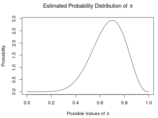
This probability distribution represents our entire estimate of \(\pi\). If we have 7 successes in 10 attempts, our estimate of the probability of different values of \(\pi\) is:

Point Estimate

As cool as the probability distribution is, it can be a little unwieldy. If we want to rank situations based on the probability of success, it would be a lot easier of we just had a number.

The single number that best estimates the value of \(\pi\) happens to be relatively easy to find. It is the expected value, or average, of our estimated probability distribution. This expected value minimizes the “mean square error”, a common measure of how far our estimate is from the actual value of \(\pi\). Because the probability distribution we found above is a beta function, we can take its parameters and plop them into what we know is the expected value of a beta function.

$$\begin{aligned} \textrm{Expected value of }\beta(y+1, n-y+1) &= \frac{y+1}{y+1+n-y+1} \\
&= \frac{1 + y}{2 + n} \\
&= \frac{1 + \textrm{Successes}}{2 + \textrm{Attempts}} \\
\end{aligned}$$

It nicely works out to a simple fraction, much like the classic estimator of \(\frac{\textrm{Successes}}{\textrm{Attempts}}\).

Improvements

Small Data Sets

Let’s see if our Bayesian point estimate works better than the classic \(\frac{\textrm{Successes}}{\textrm{Attempts}}\). Let’s say we flip a coin and it comes up heads. Here are our two estimates of the chances that a flip of this coin will come up heads.

Classic Estimate

$$\frac{\textrm{Successes}}{\textrm{Attempts}} = \frac{1}{1} = 100 \% \textrm{ chance of heads}$$

Bayesian Estimate

$$\frac{1 + \textrm{Successes}}{2 + \textrm{Attempts}} = \frac{2}{3} \approx 66 \% \textrm{ chance of heads}$$

The Bayesian estimator seems more reasonable in this situation.

Large Data Sets

What about large data sets? Lets do the same thing but with larger numbers. Let’s say we run a website that has had 1000 visitors. We know that 854 of these visitors clicked a particular link. What is our estimate of the probability a visitor will click that link?

Classic Estimate

$$\frac{\textrm{Successes}}{\textrm{Attempts}} = \frac{854}{1000} \approx 85 \%$$

Bayesian Estimate

$$\frac{1 + \textrm{Successes}}{2 + \textrm{Attempts}} = \frac{855}{1002} \approx 85 \%$$

These methods give us pretty much the same estimate.

In-Between Data Sets

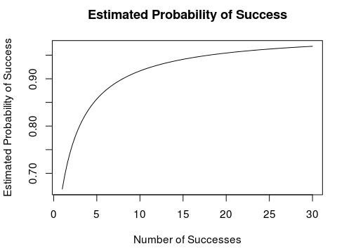
Let’s say we run a business and our first customer has been pleased with us. What is our estimate of the probability that the next customer will also be pleased? The classic \(\frac{\textrm{Successes}}{\textrm{Attempts}}\) estimator says 100%. As we get more happy customers its estimate doesn’t change. In contrast, not only is our Bayesian estimate a little more cautious to start with, but it changes as more data comes in. With each new happy customer it increases its estimate of the probability that the next customer will also be happy. If we plot this Bayesian estimate, it looks like this:

That seems to roughly follow our intuition. One happy customer doesn’t make a sure thing. But when you get 30, you figure success is actually really likely.

Conclusion

This Bayesian estimator, \(\frac{1 + \textrm{Successes}}{2 + \textrm{Attempts}}\), compares pretty well to the standard estimator, \(\frac{\textrm{Successes}}{\textrm{Attempts}}\). It estimates the probability of success more cautiously for small data sets, comes to the same conclusion for large data sets, and adjusts its estimate as it gets more data. Because of this, it is better suited to the situations we are most interested in measuring; the ones where the chance of success is unlikely to be either guaranteed or impossible.